hope.

The Messenger (Part 6)

A succinct summary of a certain period in photos and insightful quotes (according to the author’s opinion)

Individuals face a range of options each day. Some of them would result in actions, and some would be sacrificed, creating opportunity costs. Those actions also have outcomes and consequences that might change individuals’ paths. While people would act rationally and make considerations most of the time when choosing between options, there exist cases where they listen to their hearts even when the rational calculation seems convoluted and involve many aspects. At those moments, they could not mute the sounds in their heart. There are times when the options are hard to choose, and individuals might have to struggle with themselves before finally making up their minds. The challenge would be whether it is worth enough to choose the options and take the actions, considering the arising costs when taking the actions and the opportunity cost that one might lose due to selecting the option.

Commune with your own heart upon your bed, and be still.
– Psalm

It would be worth all of the time, opportunity costs, and pain, eventually. When you have your objectives that need the degree, have the passion for it, and have the seriousness, earnestness, and perseverance. It is indeed not easy, but it is rewarding.
– AK

It is worth it to keep on fighting and going all the way until it is done, no matter what.
– Tyler Joseph

In the midst of winter, I found there was, within me, an invincible summer
– Albert Camus

What you hear in your heart, let it echo this time, don’t suppress it.
What you’ve forged so far, don’t consider it worthless.
Only you know all your sacrifices for the things you love.
Ask yourself, how much you’re willing to change your life.
Various trials and things that make you doubt,
turn them into sparks to strengthen your determination.

– Hindia

A Comment on Why You Should Never Use the Hodrick-Prescott Filter

In his article, Hamilton (2017) conveyed a critique of the Hodrick-Prescott (HP) filter, arguing against its utilization due to several inherent issues. He emphasizes that the filter’s sensitivity to the smoothing parameter selection, its tendency to generate misleading cycles, and its failure to accurately represent the actual underlying trend are significant drawbacks. While I partially concur with Hamilton’s viewpoint, it is essential to note that both filters offer distinct perspectives on the cyclical characteristics of the data, and it might be interesting to rethink certain aspects of Hamilton’s arguments.

Firstly, it is argued that the HP filter leads to a series of misleading dynamic associations, which lack a foundation in the underlying data-generating process. The underlying critique of the HP filter revolves around its tendency to impose dynamic patterns that are not connected to how the data is generated. While one might accept the notion of a random walk on a trend, relying solely on asymptotic statistics may not always yield definitive results. Nonetheless, it is worth noting that such series rarely emerge, allowing the HP-detrended series to demonstrate reliable forecasting capabilities (Dritsaki & Dritsaki, 2022).

Secondly, the critique argues that the HP filter yields significantly different filtered values at the end of the sample compared to the middle, leading to spurious dynamics. However, this bias may not be a concern when detrending targets specific business cycle events and is not used for real-time analysis or macroeconomic forecasts (Dritsaki & Dritsaki, 2022). Despite these shortcomings, the HP filter can still be useful with two adjustments, a lower smoothing parameter and rescaling of the extracted cyclical component (Wolf et al., 2020). However, this point of critique is relevant to the filter’s capability to create cycles where they do not exist. Previous studies (Nelson & Kang, 1981; Cogley & Nason, 1995) have shown that linear detrending of a random walk time series can induce spurious periodicity and complex dynamic properties in cyclical components that seemingly do not exist.

Thirdly, it is argued that when statistically formalizing the problem, the smoothing parameter (𝜆) values vastly differ from common practice. Hamilton contends that for quarterly data, a 𝜆 value below 1600 results in the last component of the trend-cycle decomposition being considered white noise. He proposes estimating 𝜆 using the maximum likelihood method and advocates setting the highest value for the 𝜆 coefficient to address excessive flexibility in the trend line. Nonetheless, Schuler (2018) demonstrates that the Hamilton regression filter possesses some drawbacks in common with the Hodrick-Prescott filter, such as the cancellation of two-year cycles and the amplification of longer cycles than typical business cycles, leading to inconsistencies with typical business cycle facts recognized by the National Bureau of Economic Research Studies (NBER) Business Cycle Dating Committee.

As an alternative to the Hodrick-Prescott (HP) filter, Hamilton proposes a robust detrending approach by regressing the variable at date t+h on the four most recent values as of date t. This approach is deemed superior to the HP filter as it avoids spurious dynamic relations and dynamics, providing more stable estimates of the underlying trend. Business cycle information could be extracted directly from time series using suitably selected forecasting OLS error from an autoregression model. Moreover, the approach offers greater flexibility by involving additional variables in the regression as necessary (Dritsaki & Dritsaki, 2022).

Nevertheless, the proposed alternative filter by Hamilton faces similar criticisms as the HP filter, including the presence of filter-induced dynamics in estimated cycles and the arbitrary nature of a key parameter choice (Moura, 2022). Moreover, the Hamilton approach’s estimated trends inherently lag the data, raising doubts about its claimed superiority over the HP filter in practice. Recent empirical research also shows that the HP filter outperforms Hamilton’s filter in dynamic forecasting, with significantly smaller cycle volatilities (Dritsaki and Dritsaki, 2022). The HP or Hamilton filter would inherently produce distinct estimates of the cyclical component. However, this issue becomes less significant when relating stationary economic models to non-stationary data, as comparisons between filtered real-world data and model-filtered series are feasible (Burnside, 1998).

In conclusion, both filters offer distinct perspectives on the cyclical properties of the data, with no clear superiority. As Hodrick (2020) proposes, future research could focus on developing simultaneous multivariate econometric models that apply filters for decomposing trends and cyclical components present in economic data, influencing the development of business cycles.

References
Burnside, C. (1998). Detrending and business cycle facts: A comment. Journal of Monetary Economics, 41(3), 513-532.

Cogley, T., & Nason, J. M. (1995). Effects of the Hodrick-Prescott filter on trend and difference stationary time series: Implications for business cycle research. Journal of Economic Dynamics and Control, 19(1-2): 253-278.

Dritsaki, M., & Dritsaki, C. (2022). Comparison of HP Filter and the Hamilton’s Regression. Mathematics, 10(8):1237.

Hamilton, J. (2017, June 22). Why you should never use the Hodrick-Prescott filter. Centre for Economic Policy Research. https://cepr.org/voxeu/columns/why-you-should-never-use-hodrick-prescott-filter.

Hamilton, J. (2018). Why you should never use the Hodrick-Prescott filter. Review of Economics and Statistics, 100(5), 831-843.

Hodrick, R. J. (2020). An Exploration of Trend-Cycle Decomposition Methodologies in Simulated Data. National Bureau of Economic Research, Working Paper No. 26750.

Moura, A. (2022). Why you should never use the Hodrick-Prescott filter: Comment. MPRA Paper, No.114922

Nelson, C., & Kang, H. (1981). Spurious Periodicity in Inappropriately Detrended Time Series. Econometrica, 49, 741–751.

Schuler, Y. S. (2018). On the Cyclical Properties of Hamilton’s Regression Filter. Deutsche Bundesbank Discussion Paper 03/2018.

Wolf, E., Mokinski, F., & Schüler, Y. (2020). On Adjusting the One-Sided Hodrick–Prescott Filter. Deutsche Bundesbank Discussion Paper No. 11/2020.

Is It Worth the Waiting?

A discussion was running through my mind while I was waiting for the pick-up, thinking about a conversation with a friend lately. He mentioned being pragmatic in the context of marriage, meaning a marriage established not because of pure and true love, but rather due to other reasons, such as late age, matchmaking, etc. A couple of months ago, a friend of mine also talked about a romantic relationship that proceed to marriage because of the “easiness” factor, taking the example of a person that married his wife only after a relatively short time of dating and felt that the relationship was not complicated before deciding to get married. However, when one gets married because of other reasons instead of true love, this might raise an issue when a person appears in his life and find out he is in love with her, potentially making an affair or other relationship conflicts. Hence, the question might be whether it is worth waiting for the right person that we truly love or rather continuing our relationship in terms of marriage with another person that comes into our life that seems easy and not complicated even though we might not really love this person (assuming we aim to be in marriage sometime).

The root of the problem is not the waiting per se. It is the uncertainty of how long should we wait until we meet the right person. Just like waiting for the pick-up, we know that the pick-up will come eventually, but what time will it exactly arrive is still bewildering. A lot of reasons might make the pick-up comes late, maybe it is because of the traffic. Perhaps it is due to some technical issue, or probably it is simply not the time yet. This is a challenge to our patience in terms of waiting. We might think of choosing other transportation options as available. Nonetheless, it is only the pick-up that might be the best choice for many reasons. Should we wait? or should we make a trade-off with other transportation? There might even be another option: we could walk along our journey to the predetermined destination and take that pick-up along our way to the destination. However, we might arrive at our destination without taking the pick-up at all, or there might be many risks and challenges along the way that might be difficult for us to walk by ourselves so we need to take the pick-up.

One probability is that we might have met our significant others but have not realized it yet, or even have denied it. Should we wait, then? At this point, I guess so. There is time for us to make a move, and there is time to be patient and wait. It might be biased since I personally emphasize the value of passion and intimacy in a relationship, just like I value substantial and essential parts of a job. What is the point of doing something that we do not really enjoy only because of certain reasons? While sometimes we should be realistic and make a consideration, it might not be worth the time to do things that we do not really enjoy for most of our time. What is the point of being with someone for the rest of one’s life without having true love, passion, and intimacy with her? While there might be costs to this principle, for example, it might take time before meeting or finally getting into a serious relationship with a significant other that we truly love, not to mention the personal need of someone who could accompany us, and the social pressure, it might be worth the waiting.

As a closure, this waiting stuff reminds me of a conversation with my professor. I was asking whether it was worth it for her to pursue a doctoral degree with all of the time, opportunity costs, and “pain” as many people taking the degree said. And she said yes, it was worth it, eventually (of course, assuming we have our objectives that need the degree, have the passion for it, and have the seriousness, earnestness, and perseverance). It is indeed not easy, but it is requital.

Commentary on Monetary policy is Weaker in Recessions

In their article, Tenreyro and Thwaites (2013) conduct research to explore the impact of monetary policy on real and nominal variables at various business cycle stages. They aim to determine whether the effects of monetary policy are symmetrical or asymmetrical throughout the business cycle and identify the sources of any asymmetry observed. In my view, considering these objectives, using the impulse response functions (IRFs) in the study is quite persuasive since it is combined with other methods to complement its limitation in answering the study’s objectives.

The authors employ IRFs to analyze the dynamic response of a variable system to a specific shock. These functions capture the average effect of the shock on the system’s variables based on the state of the economy when the shock occurs, encompassing its impact on future changes. By utilizing IRFs, the authors estimate how real and nominal variables respond to monetary policy shocks, facilitating the examination of response magnitude and timing. Additionally, IRFs allow them to study variations in these responses between economic expansions and recessions.

Despite their usefulness, IRFs have some limitations. First is their assumption of linearity and exogenous shocks, which may not always hold in real-world economic systems. Their effectiveness depends on the underlying model used to generate them, and different models can yield varying IRFs. Non-linearities or structural breaks, which are significant characteristics of variable relationships, are not accounted for in IRFs, lacking a comprehensive depiction of variables’ interconnectedness. Additionally, in cases where the data-generating process cannot be adequately approximated by a vector autoregression (VAR) process, IRFs derived from the model may lead to biased and misleading results. Therefore, it is essential to consider these limitations when interpreting the implications of IRFs in economic analysis.

While IRFs are valuable for studying the dynamic impact of shocks on variable systems, they may not be the sole or optimal approach for answering the questions of the study. Hence, it is essential to complement them with other analytical tools. In this case, it is my view that Tenreyro and Thwaites have effectively utilized a combination of methods to extend the IRFs’ analysis. To complement IRFs, the authors incorporate the local projection method (Jordà, 2005), and combine it with the smooth transition regression method (Granger & Terasvirta, 1994). This adaptation allows IRFs to be influenced by the state of the business cycle, offering a more comprehensive perspective on the effects of shocks. Moreover, this combined methodology improves the estimation of shocks and reduces susceptibility to measurement errors.

The article clearly explains that the local projection method offers several advantages for studying the impact variation of shocks over time. One key advantage is their focus on the state of the economy at the time of the shock’s occurrence, lending flexibility to accommodate a panel structure and reducing sensitivity to misspecification. Furthermore, the combination method of smooth transition regression local projection model (STLPM) effectively handles non-linearities, which are weaknesses of IRFs, and estimates the impulse response of real and nominal variables to monetary policy shocks during different stages of the business cycle. In contrast, IRFs assume a constant state of the economy when the shock hits, which becomes problematic when dealing with shocks that lead to significant real effects. Estimating the transition between different economic regimes caused by the policy shock in a regime-switching VAR model involves numerous modeling choices that can be prone to errors and controversies. By employing a regime-switching local projection model, researchers avoid the need to make assumptions about how the economy transitions between regimes, which is particularly beneficial when studying the effects of fiscal consolidations or other impactful policy shocks.

Nevertheless, it should be noted that employing the local projection IRFs method tends to exhibit increased bias and variance. As a result, the confidence intervals for impulse responses are generally less accurate and wider on average compared to appropriately designed intervals based on VAR models (Kilian & Kim, 2009). Hence, in the case of a finite sample in the subsamples data in the analysis, it could hypothetically result in a wider confidence interval of IRFs. It means that using confidence intervals for IRFs in the study could shed more information about IRFs’ estimation accuracy.

Moreover, it is imperative to consider that the article’s analysis focused on the United States as an industrialized and developed country. As a result, the applicability and generalizability of the findings to emerging economies may raise some questions. Thus, future research could explore these aspects in more detail to understand how the effects of monetary policy may vary in different economic contexts.

References
Granger, C., & Terasvirta, T. (1994). Modelling nonlinear economic relationships. International Journal of Forecasting, 10(1):169–171.

Jordà, Ò. (2005). Estimation and Inference of Impulse Responses by Local Projections. American Economic Review, 95 (1): 161-182.

Kilan, L., & Kim, Y. J. (2009). Do Local Projections Solve the Bias Problem in Impulse Response Inference?. CEPR Discussion Paper Series 7266. Tenreyro, S., & Thwaites, G. (2013). Pushing on a string: US monetary policy is less powerful in recessions. CEP Discussion Paper 1218.

Revisiting Inflation Forecasts Using the ARMA

The autoregressive moving average (ARMA) is a common technique in time series analysis. In my view, a time series example that can be suitable with the ARMA model but need to be revisited is inflation. The model commonly used in inflation data modeling might associate with the relatedness of the variable with its past values. The ARMA model can be used to forecast inflation, and its simple structure that only requires current and past inflation data might offer several advantages. For example, the ARMA (p, q) model forecasts inflation at a given period by linearly projecting the inflation from the previous period to the period in question (autoregressive or AR part) and incorporating white noise from the current period to a certain number of periods back (moving average or MA part). Moreover, the ARMA model used for short-term forecasting tends to perform better on average compared to medium-term forecasting (Stovicek, 2007).

However, there are some considerations before applying the ARMA model to the inflation case. First, determining the model specification can be challenging since the ARMA model might lack a theoretical foundation. Although economic theory suggests that factors like money supply, nominal appreciation, and output gaps influence inflation, the ARMA model might not explicitly incorporate these insights. Moreover, one study found that the US CPI inflation is effectively represented by an unobserved components model with time-varying volatility in both the transitory and trend equations, implying the need to update the ARMA framework to incorporate a time-varying second moment (Stock and Watson, 2007).

Second, it is worth noting that ARMA can only be applied if the stationarity assumption holds. In the absence of stationarity in inflation data, it may be more appropriate to choose ARIMA to induce stationarity. Third, in cases where inflation occurs seasonally due to special events like Christmas or other holidays, other models might outperform ARMA. For example, previous literature suggests that SARIMA could be a better choice in such scenarios (Davidescu et al., 2021). SARIMA models offer advantages over ARIMA models when dealing with data that exhibits strong seasonal patterns, such as higher prices that can be expected during certain months due to holidays or seasonal demand. SARIMA models can capture this effect and adjust the forecasts accordingly, and can also handle multiple seasonal cycles, such as weekly, monthly, and yearly patterns.

Fourth, monetary policy interventions can also influence inflation, leading to structural shocks or breaks. It might be pivotal to consider the sample period and subset the data if necessary to ensure there are no obvious structural breaks, particularly in the case of developed economies. Inflation in advanced economies might be primarily determined by the monetary policy stance of the central bank, such as the Federal Reserve in the case of the US. Additionally, a shift in the monetary policy regime during the sample period might also indicate structural breaks in the data.

Lastly, as central banks target a specific inflation rate, an inflation series should be stationary with a long-run mean centered at the target rate. In most cases, inflation series are highly persistent due to economic reasons. Therefore, before applying Box-Jenkins forecasting techniques, inflation series are typically differenced again. In other words, forecasting is usually conducted for inflation growth rather than inflation levels. To summarize, it might be beneficial to fit various models and compare them using appropriate model selection criteria to determine the best model for inflation forecasting purposes.

References
Davidescu, A. A., Apostu, S. A., & Stoica, L. A. (2021). Socioeconomic effects of COVID-19 pandemic: exploring uncertainty in the forecast of the Romanian unemployment rate for the period 2020–2023. Sustainability, 13(13), 7078.

Stock, J. H., & Watson, M. W. (2007). Why has US inflation become harder to forecast?. Journal of Money, Credit and Banking, 39, 3-33.

Stoviček, K. (2007). Forecasting with ARMA Models: The case of Slovenian inflation. Bank of Slovenia.

Commentary on Why are Target Interest Rate Changes so Persistent?

In their paper, Coibion and Gorodnichenko (2011) argue that in the absence of additional significant economic shocks, the monetary policy reversal is likely to be gradual and provide robust evidence that policy inertia is a more likely source of the persistence in interest rates than the persistent shocks hypothesis. The author mostly agrees with their arguments for some reasons.

First, using the Taylor rule as an analytical framework is appropriate for modeling the endogenous response of monetary policymakers to economic fluctuations. Coibion and Gorodnichenko then provide a novelty and account for significant factors that affect the decision-making process by extending the classic Taylor rule to incorporate both the output gap and the output growth rate. They apply formulas that incorporate interest rate smoothing to the Taylor rule. By doing so, they find high levels of interest smoothing, indicating the presence of policy inertia and suggesting that interest rate adjustments occur gradually over time. Moreover, to explore the possibility of persistent shocks contributing to serial correlation, they assume that the errors in the baseline formula, the Taylor rule, are serially correlated. They compare the fitted values of the Taylor rule under both the policy inertia and persistent shocks interpretations and find that the fitted values for the two interpretations are essentially indistinguishable, indicating that the observed serial correlation can be attributed to policy inertia rather than persistent shocks.

Second, from a technical point of view, Coibion and Gorodnichenko (2011) address the issue of serial correlation in the error terms of the estimated Taylor rule which can lead to an overestimation of the degree of policy inertia. Hence, they provide rigorous evidence using various methods back and validate their findings and arguments. For instance, one important finding is the presence of significant policy inertia, characterized by interest rate smoothing and gradual adjustments in response to economic conditions. This evidence suggests that historical policy changes can be accounted for by interest smoothing to a significant extent, reducing the level of serial correlation in the residuals. Additionally, they explore the response of monetary policy to expected output growth, finding that adjusting for the response to expected output growth in the next quarter leads to more accurate estimates of the persistence of monetary policy shocks. These findings contribute to a better understanding of the determinants of interest rate dynamics and provide valuable insights into the behavior of the central bank.

Third, they argue that central bankers are inclined to adjust interest rates gradually and incrementally, moving them closer to their desired levels through a series of steps rather than making immediate changes as suggested by the baseline Taylor rule. This is also reaching close to the policy-making in practice where central banks typically adjust interest rates on a gradual basis. For example, the interest rate set by the central bank of Indonesia in September 2022 was 4.25%. The interest rate then gradually rose to the level of 4.75% in October 2022, 5.25% in November 2022, 5.50% in December 2022, and 5.75% in January to date (as of June 2023). The central bank made these adjustments as a response to global economic conditions and the rise in the U.S. interest rates. Finally, their points have also considered alternative factors, such as financial market variables and real-time forecast revisions, reflecting sound econometric methodology. By examining their impact on interest rate persistence and finding limited significance, the researchers demonstrate the robustness of their analysis and strengthen the case for policy inertia.

Lastly, in the author’s view, the article suggests that monetary policy can be both forward-looking and backward-looking and that the degree of policy inertia can depend on the specific formulation and the degree of interest rate smoothing in the central bank’s reaction function. If the central bank is highly responsive to past deviations of inflation from its target, then it may be slow to adjust its policy rate in response to new information about the economy, and it can be considered backward-looking. Conversely, if the central bank is more responsive to expected future deviations of inflation from its target, then it may be slow to adjust its policy rate in response to changes in the current economic environment, and it can be considered forward-looking.

References
Coibion, O., & Gorodnichenko, Y. (2011). Why are target interest rate changes so persistent?. NBER Working Papers 16707

Gorodnichenko, Y., & Coibion, O. (2011, January 28). How inertial is monetary policy? implications for the Fed’s exit strategy. CEPR. https://cepr.org/voxeu/columns/how-inertial-monetary-policy-implications-feds-exit-strategy

A Comment on How Do We Know Climate Change is Real?

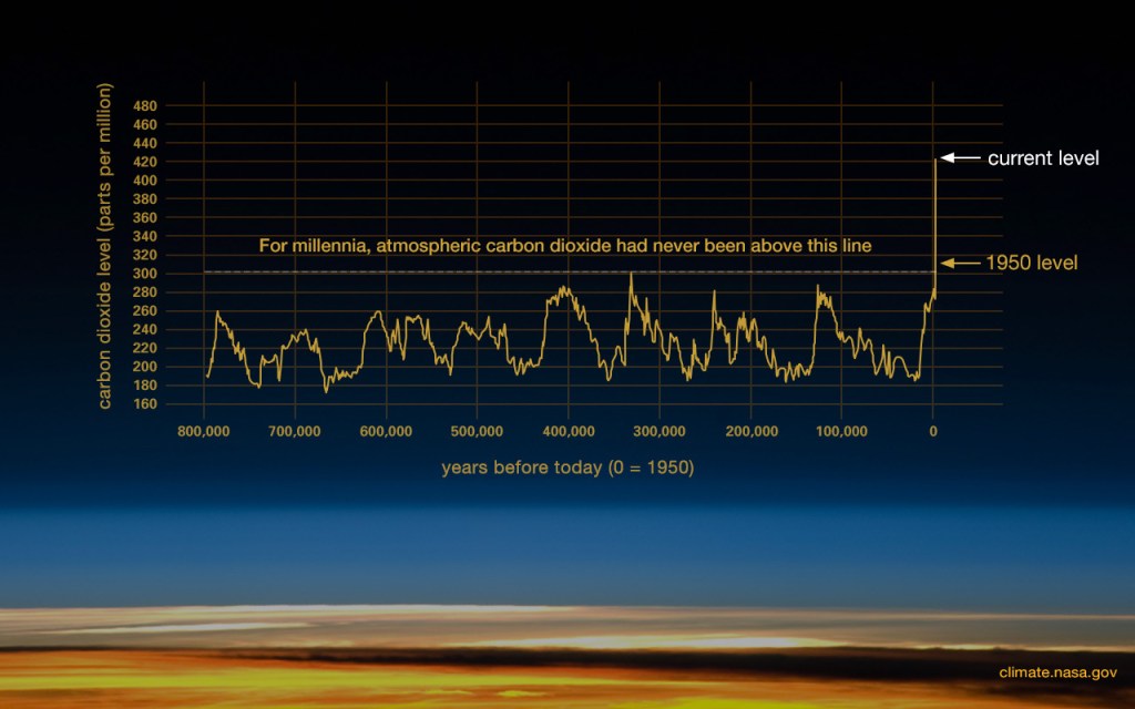
The earth has witnessed climate changes over time, but the current warming is occurring at an unprecedented pace compared to the last 10,000 years. The Intergovernmental Panel on Climate Change (IPCC) asserts that since the 1970s when systematic scientific assessments commenced, the impact of human activity on climate warming has transformed from a theoretical concept into an acknowledged reality. Nevertheless, it is quite interesting to revisit the historical data of 10,000 years provided from another perspective.

Based on a technical point of view, the dynamic behavior of carbon dioxide indicates obeying the property of the cyclical component of a time series analysis. The cycles in the carbon dioxide dynamic behavior time series data are aperiodic such that the series oscillates around the mean, but the timing and duration of the excursions above and below the mean are irregular. The series does not appear to exhibit a trend since there is no tendency for the series to increase or decrease persistently. It also does not show the seasonal component in particular since the changes in the series do not follow predictable ways of timing. In general, the cycle of the dynamic behavior of carbon dioxide tends to repeat in a span of 100,000 years.

Source: NASA (https://climate.nasa.gov/evidence)

Nevertheless, from the author’s view, it would be less likely to argue that recent carbon dioxide levels are spurious or part of a broader pattern at the current time based only on the provided data for some reasons. First, more data points after 1950 might be needed to informally identify whether the levels of carbon dioxide are spurious and to obtain a sufficient sample size to be more convincing concerning a broader pattern of a temporary shift in the dynamics of the variable. Second, a spurious correlation can happen when two variables are correlated but do not have a causal relationship. With that being said, it appears like the values of one variable cause changes in the other variable, but that is not necessarily the case. Third, a serial correlation test might need to be conducted to check whether there is a relationship between a variable and its lags or successive values. By examining autocorrelation and partial autocorrelation, one can identify patterns in the data, understand how previous values impact future values, and make predictions about future outcomes.

Moreover, based on the data and their interpretation, it could be inferred arguments both for and against a relationship between global warming and carbon dioxide levels. The argument for the relationship between global warming and carbon dioxide levels might come from the fact that as the global warming issue has raised recently, carbon dioxide levels at the same time were significantly higher than its highest rate as well as its average level in the past 10,000 years when global warming was not an issue. There might be a correlation between the two variables. Nevertheless, correlation does not imply causality, which leads to the argument against the relationship between global warming and carbon dioxide levels.

It is important to note that it needs a robust regression analysis to argue whether there exists a causal relationship between the two variables. Even after finding some evidence of the relationship based on the regression results, one should interpret carefully as there might be other factors outside the time series regression that could help explain the relationship between global warming and carbon dioxide levels. For example, some activities such as road construction and deforestation can change the reflectivity of the earth’s surface, which might lead to a higher temperature and local warming (Fahey et al., 2017). It does not mean that what one could conclude by only looking at these time series is sufficient to understand the causality and recommend policies.

In conclusion, while the current warming of the Earth’s climate is unprecedented compared to the last 10,000 years, the relationship between global warming and carbon dioxide levels is a complex issue that requires further investigation. The influence of human activity on climate warming has been established as a fact by the IPCC, but understanding the causal relationship between global warming and carbon dioxide levels necessitates robust regression analysis and consideration of other contributing factors. To formulate effective policies and interventions, a comprehensive understanding of the dynamics of climate change and its drivers is crucial which can be explored through further research and analysis on the intricate interactions between global warming, carbon dioxide levels, and other factors influencing climate change.

References
Fahey, D.W., S.J. Doherty, K.A. Hibbard, A. Romanou & P.C. Taylor. (2017). Physical drivers of climate change. In: Climate science special report: Fourth national climate assessment, volume I [Wuebbles, D.J., D.W. Fahey, K.A. Hibbard, D.J. Dokken, B.C. Stewart & T.K. Maycock (eds.)]. U.S. Global Change Research Program: Washington, DC.

NASA

The Messenger (Part 5)

A succinct summary of a certain period in photos and insightful quotes (according to the author’s opinion)

Starting again. Continuing the journey. Moving on, leaving the past behind. In practice, sometimes it is easier to say than to do. It requires at the very least a mix of courage, motivation, maturity, calmness, determination, moment, and enforcement. To always raise up after every single down. To get the self together and come back. To fall back into place.

Most of the time it’s just too difficult, too expensive, too scary. It’s only once you’ve stopped that you realize how hard it is to start again, so you force yourself not to want it. But it’s always there.
– Ted Mosby –

As a deer longs for streams of water; more than watchmen yearn for the morning.
– Psalm –

One day we’ll wake up and brush our teeth and go to work, and at some point, we’ll suddenly realize that we haven’t thought about it at all. And that’s when we’ll know we can forget.
– Saul Goodman –

It seems like once again you’ve had to greet me with goodbye.
505 – Arctic Monkeys

Tender is the night
For a broken heart
Somewhere in these eyes
Fall back into place

Fall back into place
Space Song – Beach House

On The Potential Effect of Türkiye’s Decrease in Interest Rate on Its Macroeconomic Outcomes

As the government of Türkiye has decided to lower the interest rate (Pitel, 2022), one important question that arises would be: what is the impact of the decision on the Türkiye economy? To answer the possible effect on Türkiye’s economy, the IS-LM theory in international macroeconomics can be applied as an explanation as it is a relatively simple model linking the relationship between goods, foreign exchange, and the money market. Hence, the IS-LM model could represent, explain or predict the performance of an economy. Türkiye adopted a floating exchange rate regime under which exchange rates are determined by supply and demand conditions in the market. Based on the IS-LM theory, the decline in Türkiye’s interest rate under a floating exchange rate may lead to a depreciation of the Lira, and an increase in its trade balance, investment, and total output.

In the domestic goods market, a lower interest rate could have a positive effect on the demand and an upward shift on the demand curve through an increase in investment, resulting in more output in the economy assuming ceteris paribus. The decline in interest rate makes investment less expensive, hence, it poses an increasing effect on domestic investment. However, it also means that the domestic market becomes less attractive for investors as the domestic expected return decreases. Assuming foreign return constant, the decline in domestic return would lead to an increase in the exchange rate of the Lira, meaning a depreciation of the Lira against the US dollar in the foreign exchange market. If this is the case, assuming all else equal, it can also be expected that the trade balance of Türkiye might experience an increase as the relative price of Türkiye to the rest of the world’s goods is lower in the global market that could bolster its export value.

Nevertheless, it is important to acknowledge that the IS-LM theory has certain limitations. First, it is applicable only to a short-term examination under certain assumptions, such as sticky prices and constant foreign economic circumstances, which may not always be practical in reality. Second, it fails to account for the potential repercussions of a liquidity trap in the long run. However, one cannot rule out the possibility of a liquidity trap arising, given the Turkish government’s intention to reduce its interest rate in the future. Since this theory has its constraints, it is necessary to supplement the analysis with additional theoretical frameworks to investigate the impact of Türkiye’s decrease in interest rates, especially in the long run.

First, the Fisher Effect concept can be applied to forecast that the current situation in Türkiye may lead to a further depreciation of the country’s currency, the Lira, over the long term. As prices adjust over time, inflation is likely to occur. The Fisher Effect posits that the nominal interest rate differential is equal to the expected inflation differential. Given that Türkiye’s interest rate is one of the lowest real interest rates worldwide, a reduction in interest rates is expected to result in a higher expected inflation differential with the rest of the world, leading to further depreciation of the Lira relative to the US dollar.

Furthermore, the lower interest rates may encourage Turkish citizens to hold their money in cash since there is no opportunity cost of holding money, making cash more attractive. According to the standard model of real money demand, a decrease in the nominal interest rate leads to an increase in the overall demand for money, which can result in a higher price or inflation when the growth rate of money is higher than that of real income, assuming all else equal. Additionally, if Türkiye maintains a loose monetary policy in the long run, it can be expected that the Lira will continuously depreciate, with the expected rate of depreciation equivalent to the interest differential at that time.

Second, it is worth noting that the liquidity trap could explain the effect of Türkiye’s interest rate decline if the intention to keep lowering the interest rate is implemented. This concept suggests that when a policy drives the interest rate hit the zero lower bound (ZLB), the central bank’s capacity to lower the policy rate further is exhausted. As per the case of Türkiye, the government wanted to keep applying downward pressure to market rates to calm financial markets. This policy may lead to a liquidity trap when Türkiye’s interest rate reaches zero or the ZLB if it continuously lowers its interest rate, which in turn leaves the monetary policy ineffective in intervening in the market. In this case, fiscal policy instead could be effective as it may boost the total output of the economy without crowding out effect.

In conclusion, the IS-LM theory could be utilized to examine the consequences of the Turkish government’s decision to reduce interest rates on Türkiye’s economy, but it is necessary to incorporate other theoretical frameworks to assess the long-term implications and the possibility of a liquidity trap if the interest rates continue to decrease. In the short term, the reduction of interest rates in Türkiye is likely to have an impact on the economy, leading to a depreciation of the Lira, and an increase in the trade balance, investment, and overall output. However, in the long run, as the price level adjusts, inflation and further depreciation could occur, leading to a potential liquidity trap when the interest rate reaches the zero lower bound.

References
Feenstra, R.C., & Taylor, A. M. (2016). International Macroeconomics (4th ed.). Worth Publishers.

Pitel, L. (2022, 8 June). Turkish Lira’s Slide Accelerates as Erdoğan Vows to Continue Slashing Rates. Financial Times. https://www.ft.com/content/4f56465e-d315-4502-b117-6dbd833e02e7

Revisiting the Relevance of International Macroeconomic Policy Coordination

Given the uncertainty in the current global economic situation, one question arises regarding whether international macroeconomic policy coordination is still relevant. The choice of whether to implement international macroeconomic policy coordination depends on the specific circumstances, as explained in previous literature on the topic. First, the success of cooperation and coordination principally requires the sharing of information and analysis. However, there are differing opinions regarding the need for fiscal consolidation and the extent of adjustments required in surplus countries. Consequently, achieving agreement on these issues will require a process of building trust through shared information and analysis, as well as a collaborative approach (Adam et al., 2012).

Second, cooperative responses to international macroeconomic policy coordination are also influenced by the nature of the disturbances, according to Fischer (1987). When there are positive transmission effects, different countries will require different policies to deal with a shift in demand. In the case of a worldwide disturbance, similar policy responses will be needed in different countries if transmission effects are positive. The objectives of each country also affect the specific policy actions that should be taken. For example, the breakdown of the Bretton Woods system indicates that international differences in policy goals may be too significant for systematic macroeconomic policy coordination among major economies. Nevertheless, occasional agreements and coordination on specific policy packages may still be feasible.

Third, the exchange rate regime is a crucial factor that determines policy interactions as part of international macroeconomic policy coordination between countries. Flexible exchange rates, for instance, can provide countries with insulation from external shocks and more freedom to pursue domestic goals without worrying about foreign reactions or policies, as argued by Fischer (1987). Given the flexibility of exchange rates, it is unlikely that macroeconomic policy coordination among major economies will progress beyond the exchange of information and occasional agreements on specific policy tradeoffs. However, both information sharing and occasional policy agreements under the right circumstances are beneficial and should be encouraged. It should be noted that interdependence has still increased within the flexible rate system. In practice, the slow adjustment of domestic prices and wages assuming prices and wages are sticky in the short run, coupled with the quick adjustment of the exchange rate to policy changes, means that changes in monetary and fiscal policies in one country can rapidly affect the real exchange rate. Additionally, expansionary domestic policies could lead to the anticipation of devaluation, massive capital outflows, and eventually devaluation or a change in policies. Hence, expansionary monetary policy in one country could cause inflation and depreciation of its currency, without necessarily affecting other economies.

Fourth, it is worth considering the fiscal and monetary policy aspects in international macroeconomic policy coordination. Frankel (2015) argues that from a fiscal policy perspective, there is an assumption that fiscal stimulus has positive “spillover effects” on trading partners. Each country may be hesitant to undertake fiscal expansion alone due to concerns about worsening its trade balance, but global conditions could improve if major countries agree to work together as locomotives, pulling the global economy out of a recession. However, despite the popularity of the locomotive theory, coordination does not necessarily mean expansion across the board, as Fischer (1987) points out. The optimal cooperative policies depend on the objectives of policymakers, the nature of the transmission mechanism between the economies, the policy tools at their disposal, and the nature of the disturbances that call for policy responses. Another concern is that policies may be transmitted asymmetrically between countries.

When it comes to monetary policy, regular meetings between officials can be beneficial. For instance, consultation can reduce unexpected events, and in times of crisis, cooperation and exchange of views can help bridge gaps in perceptions. However, some calls for international coordination may be less effective, especially when they attempt to blame other countries in order to divert attention away from domestic issues and disagreements. In other words, calls for coordination can sometimes be misused to conceal domestic problems.

It is imperative to note that with greater economic integration across countries, particularly via the capital account, and asymmetries in exchange rate systems, relying on automatic adjustment mechanisms of the non-system is no longer a practical solution (Adam et al., 2012). Therefore, it is necessary to re-establish policy cooperation to rebalance the global economy and mitigate the negative spillover effects that may result from uncoordinated attempts at rebalancing.

In the long run, there may be an opportunity for countries to coordinate their policies for mutual benefit, as their understanding of policy operations and interdependence grows. While coordination is generally considered better, empirical evidence suggests that the benefits may be relatively insignificant due to the limited impact of policies in one country on others (Fischer, 1987). Additionally, differing views on policy outcomes and uncertainties about their effects may make it difficult to reach an agreement. Thus, the appropriate approach after all might be for each country to focus on keeping its economy stable, at least in the short run.

References
Adam, C., Subacchi, P., and Vines, D. (2012). International Macroeconomic Policy Coordination: An Overview. Oxford Review of Economic Policy, vol. 28, no. 3, pp. 395–410.

Fischer, S. (1987). International Macroeconomic Policy Coordination. NBER Working Papers 2244.

Frankel, J. (2015). International macroeconomic policy coordination. VoxEU CEPR.